PRML上巻 P14
昨日の続き
確率変数の確率分布を単に
と書き,その分布が特定の値
を取る確率を
と書くことにする.
このような簡潔な記法を使うと,確率論の2つの基本法則を以下のように書くことができる.
確率の基本法則
ここで,は同時確率,
は条件付き確率,
は周辺確率(単に
の確率)である.
乗法定理及び対称性から,条件付き確率の間の以下の関係を得る.
これはベイズの定理(Bayes' theorem)と呼ばれ,パターン認識や機械学習において中心的役割保果たす.
加法定理を使えば,ベイズの定理の分母は分子に現れる量を使って表すことができる.
すなわち,
と表せる.
すべてのについて和を取ると,
となる.
つまり,ベイズの定理の分母は式の左辺の条件付き確率をすべての
について和をとったものが1になることを保証するための規格化(正規化)定数とみなすことができる.
今日はここまで.
PRML上巻 P13
昨日の続き.
列の事例数は,その列にある枠内の事例数の総和のため,
である.
と
より,
が成り立つ.これが確率の加法定理(sum rule)である.
は他の変数についての周辺化,すなわち
についての足し合わせであるため,
周辺確率(marginal probability)と呼ばれることもある.
の事例だけを考え,その中での
の事例の比率を
と書き,
が与えられた下での
の条件付き確率 (conditional probability)と呼ぶ.
これは列の点の中で
の枠内にある点の数の比率であるため,
となる.
,
および
から次の関係を得る.
これは確率の乗法定理(product rule)である.
今日はここまで.
PRML上巻 P11-13
1.2 確率論
確率論(probability theory)は,不確実性に関する定量化と操作に関して一貫した枠組みを与え,パターン認識の基礎の中心を担っている.
確率に関する2つの基本的な法則がある.
- 確率の加法定理(sum rule of probability)
- 確率の乗法定理(product rule of probability)
2つの確率変数を考える.
は任意の値
,
は任意の値
を取れるものとする.
と
の両方についてサンプルを取り,全部で
回の試行を行う.そのうち
となる
試行の数を
とする.また,
が値
を取る試行の数を
,
が値
を取る試行の数を
とする.
このとき,が
,
が
を取る確率を
と書き,
と
の同時確率(結合確率; joint probability)と呼ぶ.
これは,という枠内の中にある点の個数を点の総数で割った数であるため,
で与えられる.
同様に,が
を取る確率を
と書くと,
列にある点の数を点の総数で割った数で,
となる.
眠いのでここまで.
PRML上巻 P10-11
昨日の続き.
多項式曲線フィッティングの線形方程式verを作成した.
動作確認のため,図を再描画してみる.
%matplotlib inline
import matplotlib.pyplot as plt
import numpy as np
import numpy.polynomial.polynomial as poly
np.random.seed(42)
# test data set (N=15)
# t = sin(2 \pi x) + gaussian noise
x4 = np.linspace(0, 1, 15)
t4 = np.sin(2 * np.pi * x4) + np.random.normal(0, 0.2, 15)
# test data set (N=100)
# t = sin(2 \pi x) + gaussian noise
x1 = np.linspace(0, 1, 100)
t3 = np.sin(2 * np.pi * x1) + np.random.normal(0, 0.2, 100)
# figure 1.6

def polyfit_linear_equation(x: np.ndarray, t: np.ndarray, M: int) -> np.ndarray:
    """solve linear equation

    Args:
        x (np.ndarray): explanatory variable (N dims)
        t (np.ndarray): response variable (N dims)
        M (int): order

    Returns:
        np.ndarray: coefficient (M dims)
    """
    # add intercept term
    M += 1
    # A: M x M matrix
    A = np.zeros(shape=(M, M))
    for i in range(M):
        for j in range(M):
            A[i][j] = np.sum(np.power(x, i + j))
    # T: 1 x M vector
    T = np.zeros(M)
    for i in range(M):
        T[i] = np.dot(np.power(x, i), t)
    # fitting with linear equations
    # FIXME: the result is flipped. To make the result in proper order, we must flip it.
    return np.linalg.solve(A, T)[::-1]

# fitting with polynomial functions
w9_15 = polyfit_linear_equation(x4, t4, 9)
w9_100 = polyfit_linear_equation(x1, t3, 9)

# visualize
fig, axs = plt.subplots(1, 2, figsize=(12, 4))
axs[0].set_title('N = 15')
axs[1].set_title('N = 100')

for ax in axs.flat:
    ax.plot(x1, t1, color='green')
    ax.set(xlabel='x', ylabel='t')

axs[0].scatter(x4, t4, facecolor='None', edgecolor='blue')
axs[0].plot(x1, np.poly1d(w9_15)(x1), color='red')
axs[1].scatter(x1, t3, facecolor='None', edgecolor='blue')
axs[1].plot(x1, np.poly1d(w9_100)(x1), color='red')

plt.tight_layout()

正しく動作しているようだ.
あらためて,線形方程式verを用いて図を描画してみる.
なお,正則化した線形方程式には,演習問題1.2の解答である次式を用いる.
# figure 1.7

def polyfit_linear_equation_regularize(x: np.ndarray, t: np.ndarray, M: int, alpha: float) -> np.ndarray:
    """solve linear equation

    Args:
        x (np.ndarray): explanatory variable (N dims)
        t (np.ndarray): response variable (N dims)
        M (int): order
        alpha (float): regularization parameter

    Returns:
        np.ndarray: coefficient (M dims)
    """
    # add intercept term
    M += 1
    # A: M x M matrix
    A = np.zeros(shape=(M, M))
    for i in range(M):
        for j in range(M):
            A[i][j] = np.sum(np.power(x, i + j))
    # I: M x M identity matrix
    I = np.identity(M)
    # T: 1 x M vector
    T = np.zeros(M)
    for i in range(M):
        T[i] = np.dot(np.power(x, i), t)
    A_reg = A - alpha * I
    # fitting with linear equations
    # FIXME: the result is flipped. To make the result in proper order, we must flip it.
    return np.linalg.solve(A_reg, T)[::-1]
w9_l18 = polyfit_linear_equation_regularize(x4, t4, 9, np.exp(-18))
w9_l0 = polyfit_linear_equation_regularize(x4, t4, 9, np.exp(0))
# visualize
fig, axs = plt.subplots(1, 2, figsize=(12, 4))
axs[0].set_title(r'$\ln{\lambda} = -18$')
axs[1].set_title(r'$\ln{\lambda} = 0$')

for ax in axs.flat:
    ax.plot(x1, t1, color='green')
    ax.set(xlabel='x', ylabel='t')

axs[0].scatter(x2, t2, facecolor='None', edgecolor='blue')
axs[0].plot(x1, np.poly1d(w9_l18.flatten())(x1), color='red')
axs[1].scatter(x2, t2, facecolor='None', edgecolor='blue')
axs[1].plot(x1, np.poly1d(w9_l0.flatten())(x1), color='red')

plt.tight_layout()

(元々のデータが書籍記載のものと異なるためか,書籍記載の図を再現できていない.の値を変化させて確認したところ,正則化自体はうまく動作しているようだった.よってこの図はこのままとする.)
図から,によって過学習が抑制され,背後の関数
に近い表現が得られることがわかる.ただし,
の値を大きくしすぎると図
の右側に示すように当てはまりは再び悪くなる.
正則化が期待通り係数が大きい値を取らないようにしているかを見るために,当てはめた多項式の係数を次表に示す.(コードは省略)
| |
|
|
|
|---|---|---|---|
| |
20812.84 | -2005.15 | -0.95 |
| |
-92408.71 | 3634.86 | -0.85 |
| |
170879.63 | 614.50 | -0.71 |
| |
-170219.15 | -3401.47 | -0.54 |
| |
98565.04 | -1228.53 | -0.31 |
| |
-33325.18 | 4548.16 | -0.02 |
| |
6273.03 | -2740.68 | 0.37 |
| |
-609.66 | 618.99 | 0.84 |
| |
32.65 | -40.79 | 1.19 |
| |
-0.38 | 0.20 | -0.38 |
表より,の値を増やすと共にほとんどの係数は小さな値を取るようになることがわかる.
正則化項が汎化誤差に与える影響は,訓練集合とテスト集合の両方に対するRMS誤差の値を
に対してプロットしてみれば良い.これを図
に示す.
# figure 1.8

RMSE_reg_train = []
RMSE_reg_test = []
w_values_reg = []
for alpha in range(-380, -199):
    w = polyfit_linear_equation_regularize(x2, t2, 9, np.exp(alpha / 10))
    w_values_reg.append(w.flatten())
    y_train = np.poly1d(w.flatten())(x2)
    y_test = np.poly1d(w.flatten())(x1)
    E_train = 0.5 * np.sum(np.square(y_train - t2))
    E_test = 0.5 * np.sum(np.square(y_test - t3))
    RMSE_reg_train.append(np.sqrt(2 * E_train / t2.size))
    RMSE_reg_test.append(np.sqrt(2 * E_test / t3.size))
ln_alpha = np.linspace(-38, -19, 181)
p1 = plt.plot(ln_alpha, RMSE_reg_train, color='blue')
p2 = plt.plot(ln_alpha, RMSE_reg_test, color='red')
plt.xlabel(r'$\ln{\lambda}$')
plt.ylabel(r'$E_{RMS}$')
plt.ylim(0, 1)
plt.legend([p1[0], p2[0]], ['訓練', 'テスト'])

むむ.書籍と随分違うグラフになってしまった.
このグラフから何か読み取るのは困難だが,本来は,テスト誤差が最小となるような正則化パラメータを探索すればよい,ということになるはずである.
モデルの複雑さの問題は重要で,誤差関数を最小にするようなアプローチで実際の応用問題を解こうとする際には,モデルの複雑さを適切に決める方法を見つけなければならない.
そのためには,得られたデータを,係数を決めるために使われる訓練集合と,それとは別の確認用集合(検証用集合; validation set)に分ける方法がある.確認用集合はホールドアウト集合(hold-out set)とも呼ばれ,モデルの複雑さ(
または
)を最適化するのに使われる.
これまでの多項式曲線フィッティングの議論は,主として直感に訴えるものであった. ここからは,確率論的な議論の枠組みを使い,パターン認識における問題を解くためのより原理的なアプローチを探っていく.
以上.
PRML上巻 P9
昨日の続き.
過学習を制御するためによく使われるテクニックに正則化(regularization)がある.
これは誤差関数にpenalty項を付加することにより係数が大きな値になることを防ごうとするものである.
最も単純なものは,係数を二乗して和をとったもの(L2正則化)で,誤差関数は以下となる.
ここで,であり,係数
は正則化項と二乗誤差の和の項との相対的な重要度を調整している.(ただし,係数
は正則化から外すことも多い)
このようなテクニックは統計学の分野で縮小推定(shrinkage)と呼ばれている. 特に2次の正則化の場合はリッジ回帰(ridge regression)と呼ばれる. ニューラルネットワークの文脈では荷重減衰(weight decay)として知られている.
演習問題 1.2
正則化された二乗和誤差関数を最小にする係数
が満たす,
に類似した線型方程式系を書き下せ.
演習問題 1.2 解答
に
を代入する.
が最小のとき,
の
についての偏微分が0となる.よって,
ここで,
を用いた.
演習問題 1.1 解答より,
なので,これをに代入すると.
上式のを移行すると,
に似た次式が得られる.
本日は以上.
PRML上巻 P8
昨日の続き.
いろいろな次数の多項式について得られた係数の値を検証してみる.
(コードは省略)
| 0.09 | -1.36 | 21.09 | 524.49 | |
| 0.77 | -31.88 | -8747.08 | ||
| 10.88 | 30200.27 | |||
| 0.01 | -46656.18 | |||
| 38429.23 | ||||
| -17576.78 | ||||
| 4319.81 | ||||
| -522.06 | ||||
| 28.31 | ||||
| 0.10 |
の増加に伴って,係数の多くが大きな値をとるようになっている.
次に,モデルの次数は固定し,データ集合のサイズを変えてみたときの振る舞いを確認する. (一時変数名が適当ですいません)
%matplotlib inline
import matplotlib.pyplot as plt
import numpy as np
import numpy.polynomial.polynomial as poly
np.random.seed(42)
# test data set (N=15)
# t = sin(2 \pi x) + gaussian noise
x4 = np.linspace(0, 1, 15)
t4 = np.sin(2 * np.pi * x4) + np.random.normal(0, 0.2, 15)
# test data set (N=100)
# t = sin(2 \pi x) + gaussian noise
x1 = np.linspace(0, 1, 100)
t3 = np.sin(2 * np.pi * x1) + np.random.normal(0, 0.2, 100)
# figure 1.6
# fitting with polynomial functions
w9_15 = np.polyfit(x4, t4, 9)
w9_100 = np.polyfit(x1, t3, 9)

# visualize
fig, axs = plt.subplots(1, 2, figsize=(12, 4))
axs[0].set_title('N = 15')
axs[1].set_title('N = 100')

for ax in axs.flat:
    ax.plot(x1, t1, color='green')
    ax.set(xlabel='x', ylabel='t')

axs[0].scatter(x4, t4, facecolor='None', edgecolor='blue')
axs[0].plot(x1, np.poly1d(w9_15)(x1), color='red')
axs[1].scatter(x1, t3, facecolor='None', edgecolor='blue')
axs[1].plot(x1, np.poly1d(w9_100)(x1), color='red')

plt.tight_layout()

図から,データ集合のサイズが大きくなるにつれて過学習の問題は深刻でなくなってくることがわかる.
大雑把な経験則としては,データの点の数はモデル中の適応パラメータの数の何倍か(例えば5とか10)よりは小さくてはいけない,といわれているらしい.
今日はここまで.
PRML上巻 P6-7
昨日の続き.

図をみると,次数
のケースは関数
の表現としては明らかに不適切であることがわかる.
このような振る舞いは過学習(over-fitting)として知られている.
我々の目標は,新たなデータに対して正確な予測を行える高い汎化性能の達成である.
そこで汎化性能がにどう依存するかを定量的に評価する.
テスト集合に対して,誤差関数を評価する.このとき,
で定義される平均二乗平方根誤差(root-mean-square error, RMS error)を用いると便利なことがある.
で割ることによりサイズの異なるデータ集合を比較できるようになり,平方根を取ることによって
は目的変数
と同じ尺度であることが保証される.
いろいろなに対する訓練集合とテスト集合のRMS誤差のグラフを描いてみる.
ここで,テスト集合は新たに生成した100個のデータ点からなる.
%matplotlib inline
import matplotlib.pyplot as plt
import japanize_matplotlib
import numpy as np
import numpy.polynomial.polynomial as poly
np.random.seed(42)
# t = sin(2 \pi x)
x1 = np.linspace(0, 1, 100)
t1 = np.sin(2 * np.pi * x1)
# training data set (N=10)
# t = sin(2 \pi x) + gaussian noise
x2 = np.linspace(0, 1, 10)
t2 = np.sin(2 * np.pi * x2) + np.random.normal(0, 0.2, 10)
# test data set (N=100)
# t = sin(2 \pi x) + gaussian noise
t3 = np.sin(2 * np.pi * x1) + np.random.normal(0, 0.2, 100)
RMSE_train = []
RMSE_test = []
for m in range(10):
    w = np.polyfit(x2, t2, m)
    y_train = np.poly1d(w)(x2)
    y_test = np.poly1d(w)(x1)
    E_train = 0.5 * np.sum(np.square(y_train - t2))
    E_test = 0.5 * np.sum(np.square(y_test - t1))
    RMSE_train.append(np.sqrt(2 * E_train / t2.size))
    RMSE_test.append(np.sqrt(2 * E_test / t1.size))
M = np.linspace(0, 9, 10)
p1 = plt.plot(M, RMSE_train, color='blue', marker='o', markerfacecolor='None', markeredgecolor='blue')
p2 = plt.plot(M, RMSE_test, color='red', marker='o', markerfacecolor='None', markeredgecolor='red')
plt.xlabel('M')
plt.ylabel(r'$E_{RMS}$')
plt.legend([p1[0], p2[0]], ['訓練', 'テスト'])
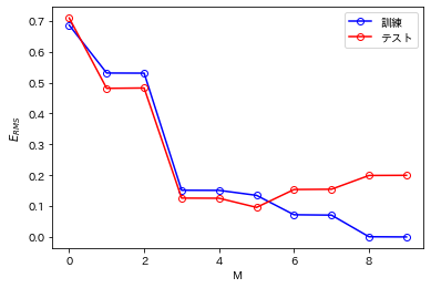
上図をみると,(書籍の図ほど顕著ではないものの)3<Mの範囲で徐々にテスト誤差が大きくなっていることがわかる.
また,では訓練誤差が0になっている.これは多項式の自由度が10であり,訓練集合の10個のデータ点にちょうど当てはめられるからである.
今日はここまで.